- Use Amazon CodeCommit. It’s the only service for multi-gigabyte repositories.
- Use Buildbot for automatic daily merges from master e.g. ironframe-buildbot.
- Push daily diffs to github via a Buildbot task e.g. diffs.
Old Project – TexGame
I uploaded a project, TexGame, from when I was 17 & 18 years old to github, it’s at https://github.com/bjwbell/texgame.
The code is in Python and uses PyGame for the graphics and sound.
The purpose of the game is to get as high a score as possible. To achieve this lines are eaten away. There is an eater block that goes across the screen. The rate at which it eats blocks depends on how many spaces it encounters. The more open spaces it eats the slower it moves, which is bad.
Menu Screen:
Playing: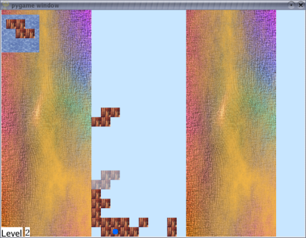
Old Project – World Racer
I uploaded a project, World Racer, from my teenager years to github. I apologize for the terrible spelling in the code, back then I had no idea how to spell almost anything.
I’ve looked at the code and it’s not bad. I’m surprised by how good of a C++ & 3d graphics programmer I was for the very first project I ever did.
The code is on github at https://github.com/bjwbell/WorldRacer.
Screenshot: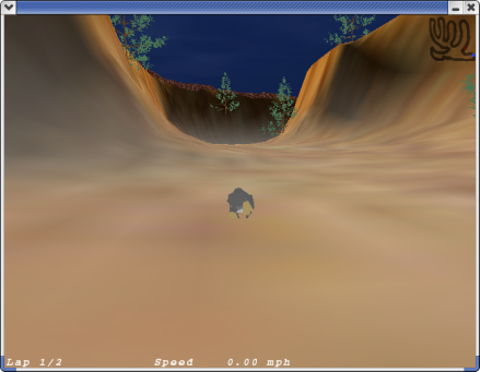
Emacs Rust Debugging
Rust-GDB
Use rust-gdb to launch gdb with the Rust-specific pretty-printers enabled, PR#19954 – add rust-gdb for Rust pretty printers.
GDB Rust Breakpoints
In gdb use break FILENAME:LINE_NUM instead of rbreak FUNCTION_NAME.
Rust has lifetime parameters, which can cause the gdb error umatched quote.
Example
Code: struct Foo<‘a> {num: i32} impl<‘a> Foo<‘a> { fn add_one(self) {} }
GDB:
    (gdb) rbreak add_one

     unmatched quote

    (gdb)
Emacs GUD
- To Launch: M-x gdb
- Instead of gdb enter rust-gdb, add –-args to pass arguments to the proccess being debugged.
- Example:
rust-gdb --i=mi --args PATH_TO_EXECUTABLE EXECUTABLE_ARGS
Emacs GUD – Keybindings
I never remember the Emacs GUD keybindings, instead my .emacs includes:
(global-set-key [f5] 'gud-cont)

(global-set-key [f7] 'gud-tbreak)

(global-set-key [S-f11] 'gud-finish)

(global-set-key [f9] 'gud-break)

(global-set-key [f10] 'gud-next)

(global-set-key [f11] 'gud-step)
Emacs Rust Development Setup
========BASIC SETUP===========
- Basic support, e.g. syntax highlighting – instructions @ rust-mode.
- Source code tagging – Exuberant Ctags + copy ctags.rust to $HOME/.ctags
- On the fly syntax checking – flymake-rust.
- Code completion – racer.
=======PROJECT SETUP==========
Read the Cargo guide.
=======GGTAGS SETUP==========
For cross referencing via ggtags:
- Download and install Gnu Global (the Gnu Global package available in Ubuntu 14.04 doesn’t allow adding new lang defs).
- Ensure that $HOME/.ctags includes the Rust lang definitions from ctags.rust.
- Set the env variable GTAGSCONF to $HOME/.globalrc
- Set the env variable GTAGSLABEL to ctags, e.g. export GTAGSLABLE=”ctags”
- Sometimes eshell in emacs doesn’t inherit the env variables, in which case run gtags . in a normal shell.
- To .emacs add
(add-hook 'prog-mode-hook '(lambda () (when (derived-mode-p 'rust-mode) (ggtags-mode 1)))) - Copy to .globalrc
# Configuration file for GNU GLOBAL source code tag system.
#
# Basically, GLOBAL doesn't need this file ('gtags.conf'), because it has
# default values in its self. If you have the file as '/etc/gtags.conf' or
# "$HOME/.globalrc" in your system then GLOBAL overwrite the default values
# with the values in the file.
#
# The format is similar to termcap(5). You can specify a target with
# GTAGSLABEL environment variable. Default target is 'default'.
#
default:\
	:tc=native:
native:\
	:tc=gtags:
ctags:\
	:tc=exuberant-ctags:
#---------------------------------------------------------------------
# Configuration for gtags(1)
# See gtags(1).
#---------------------------------------------------------------------
common:\
	:skip=HTML/,HTML.pub/,tags,TAGS,ID,y.tab.c,y.tab.h,gtags.files,cscope.files,cscope.out,cscope.po.out,cscope.in.out,SCCS/,RCS/,CVS/,CVSROOT/,{arch}/,autom4te.cache/,*.orig,*.rej,*.bak,*~,#*#,*.swp,*.tmp,*_flymake.*,*_flymake:
#
# Built-in parsers.
#
gtags:\
	:tc=common:\
	:tc=builtin-parser:
builtin-parser:\
	:langmap=c\:.c.h,yacc\:.y,asm\:.s.S,java\:.java,cpp\:.c++.cc.hh.cpp.cxx.hxx.hpp.C.H,php\:.php.php3.phtml:
#
# Plug-in parser to use Exuberant Ctags.
#
exuberant-ctags|plugin-example|setting to use Exuberant Ctags plug-in parser:\
	:tc=common:\
	:langmap=Asm\:.asm.ASM.s.S:\
	:langmap=Awk\:.awk.gawk.mawk:\
	:langmap=C\:.c:\
	:langmap=C++\:.c++.cc.cp.cpp.cxx.h.h++.hh.hp.hpp.hxx.C.H:\
	:langmap=Flex\:.as.mxml:\
	:langmap=HTML\:.htm.html:\
	:langmap=Java\:.java:\
	:langmap=JavaScript\:.js:\
	:langmap=Lisp\:.cl.clisp.el.l.lisp.lsp:\
	:langmap=Perl\:.pl.pm.plx.perl:\
	:langmap=Python\:.py.pyx.pxd.pxi.scons:\
	:langmap=Ruby\:.rb.ruby:\
        :langmap=Rust\:.rs:\
	:langmap=Scheme\:.SCM.SM.sch.scheme.scm.sm:\
	:langmap=Sh\:.sh.SH.bsh.bash.ksh.zsh:\
	:langmap=YACC\:.y:\
	:gtags_parser=Asm\:/usr/local/lib/gtags/exuberant-ctags.la:\
	:gtags_parser=Awk\:/usr/local/lib/gtags/exuberant-ctags.la:\
	:gtags_parser=C\:/usr/local/lib/gtags/exuberant-ctags.la:\
	:gtags_parser=C++\:/usr/local/lib/gtags/exuberant-ctags.la:\
	:gtags_parser=Flex\:/usr/local/lib/gtags/exuberant-ctags.la:\
	:gtags_parser=HTML\:/usr/local/lib/gtags/exuberant-ctags.la:\
	:gtags_parser=Java\:/usr/local/lib/gtags/exuberant-ctags.la:\
	:gtags_parser=JavaScript\:/usr/local/lib/gtags/exuberant-ctags.la:\
	:gtags_parser=Lisp\:/usr/local/lib/gtags/exuberant-ctags.la:\
	:gtags_parser=Perl\:/usr/local/lib/gtags/exuberant-ctags.la:\
	:gtags_parser=Python\:/usr/local/lib/gtags/exuberant-ctags.la:\
	:gtags_parser=Ruby\:/usr/local/lib/gtags/exuberant-ctags.la:\
        :gtags_parser=Rust\:/usr/local/lib/gtags/exuberant-ctags.la:\
	:gtags_parser=Scheme\:/usr/local/lib/gtags/exuberant-ctags.la:\
	:gtags_parser=Sh\:/usr/local/lib/gtags/exuberant-ctags.la:\
	:gtags_parser=YACC\:/usr/local/lib/gtags/exuberant-ctags.la:
======================TIPS======================
Usable keyboard shortcuts for navigation, with Rust code:
- M-. – ggtags-find-tag-dwim – Go to definition
- C-c M-g – ggtags-grep – Grep for references
Bind ggtags-grep to “M-]”, for finding references:
(add-hook 'prog-mode-hook
      '(lambda ()
         (when (derived-mode-p 'rust-mode)
           (define-key ggtags-mode-map (kbd "M-]") 'ggtags-grep)
           )))
Implementing the Closest Pair Algorithm in OpenCL and WebCL
I was looking for a fun geometry problem to solve and came across the closest pair of points problem.
The problem statement is:
Given a set of points, in 2D, compute the closest pair of points.
The brute force algorithm takes 

As far as I know, there aren’t any posted solutions using OpenCL to compute the closest pair. So I’ve implemented one, it’s posted at closest-pair.
There are a few challenges in adapting the algorithm for OpenCL. Namely, we can’t use recursion so we must convert the recursive algorithm to a procedural one. In this case it’s not to complicated because the structure of the solution is easily converted from the top-down recursive algorithm to a bottom-up parallel algorithm. There are some tricky issues when the number of points are not a power of 2. I’ve commented the code for those cases.
The second challenge is using WebCL. WebCL has an additional restriction that you can’t pass structures between Javascript and OpenCL kernels. Because of this I had to use dumb arrays of simple uint’s instead of using arrays of uint2, uint3, and uint4. This made the code more verbose. To help reduce the verbosity I added macros in the OpenCL ckStrips kernel. The WebCL version is posted at
closest_pair_ocl.html.
I hope the solution is useful to someone. Enjoy reading the code, it requires careful thought.
Check it out at closest-pair or view the WebCL one online at closest_pair_ocl.html.
Enabling WebCL Highlighting in Emacs
When editing WebCL OpenCL kernels in Emacs I like to have the OpenCL kernel code highlighted as C code. This is easy to achieve using the multi-mode.el package.
The steps on Ubuntu (or any other modern Linux with Emacs 24) are
- Enable the http://marmalade-repo.org/ elpa package archive by adding the below to your .emacs file and restarting Emacs
(require 'package) (add-to-list 'package-archives '("marmalade" . "http://marmalade-repo.org/packages/")) (package-initialize) - Install multi-web-mode by using “M-x package-list-packages” and scrolling down to “multi-web-mode”.
- Add the below to the bottom of your .emacs file and restart Emacs
    (require 'multi-web-mode)
    (setq mweb-default-major-mode 'html-mode)
    (setq mweb-tags '((php-mode "<\\?php\\|<\\? \\|")
                      (js-mode "]*>" "")
                      (css-mode "]*>" "")
	              (c-mode "]* +type=\"text/x-opencl\"[^>]*>" "")))
    (setq mweb-filename-extensions '("php" "htm" "html" "ctp" "phtml" "php4" "php5"))
    (multi-web-global-mode 1)
The important part is the “c-mode” section that will enable C highlighting for OpenCL kernels in html files.
- Start coding!
Computing the Smallest Enclosing Disk
I recently read in chapter 4 of Computational Geometry by de Berg et al. the problem of computing the smallest enclosing disk for a set of points.
I’ve shamelessly stolen the algorithm from there and done a simple conversion to Javascript.
The code is under the canvas-geolib GitHub repository in the geometry.js file, there’s also an example @ enclosingdisk.html. The example initially consists of three points and the smallest disk enclosing them. Click anywhere on the canvas and a new point will be added and the disk redrawn.
I don’t want to go over the general algorithm but I do want explain computing the unique disk with three points given for its boundary. In geometry.js the function “enclosingDisk3Points” takes three points and returns the unique disk that has those points on its boundary.
The below figure shows the two defining characteristics of the disk, which are (1) the disk center is centered at (x,y) and (2) the distance from the center to all three points (p0, p1, & p3) is equal i.e. the distance from the center to all three points is d.
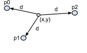
From this computing (x,y) and d is simple. For simplicity we assume 


The set of equations to solve is:


Solving for y, we have 


The below Javascript code implements the above computation and also adds the preprocessing steps of (1) translating the origin to 


// return the unique disk with p1, p2, and p3 as boundary points.
function enclosingDisk3Points(_p1, _p2, _p3){

    var p1 = [_p1[0], _p1[1]];
    var p2 = [_p2[0], _p2[1]];
    var p3 = [_p3[0], _p3[1]];
    if (dist(p1, p3) > dist(p1, p2)){
var p = p2;
p2 = p3;
p3 = p;
    }

    var p = p1;
    // make p1 the origin
    p2[0] = p2[0] - p1[0];
    p2[1] = p2[1] - p1[1];
    p3[0] = p3[0] - p1[0];
    p3[1] = p3[1] - p1[1];

    // apply rotation matrix to make p2.x = 0
    // the rotation matrix is
    // | p2[1]/dist(p2), -1 * p2[0]/dist(p2) |
    // | p2[0]/dist(p2), p2[1]/dist(p2) |
    //
    var original_p2 = [p2[0], p2[1]];
    p2[0] = 0;
    p2[1] = d(original_p2);

    // apply rotation matrix to p3
    var original_p3 = [p3[0], p3[1]]
    p3[0] = original_p2[1]/d(original_p2) * original_p3[0] - original_p2[0]/d(original_p2) * original_p3[1]
    p3[1] = original_p2[0]/d(original_p2) * original_p3[0] + original_p2[1]/d(original_p2) * original_p3[1]

    // the unique disk with the points p1, p2, and p3 as boundary points is
    // defined by the equation y = p2.y/2 & x = (d(p3)^2 + p3.y * p2.y)/(2 * p3.x)
    var y = p2[1]/2.0;
    var x = (d(p3) * d(p3) - p3[1] * p2[1])/(2 * p3[0]);

    // apply inverse of rotation matrix
    var rotated_x = original_p2[1]/d(original_p2) * x + original_p2[0]/d(original_p2) * y
    var rotated_y = -1 * original_p2[0]/d(original_p2) * x + original_p2[1]/d(original_p2) * y;

    // translate back
    rotated_x = rotated_x + p1[0];
    rotated_y = rotated_y + p1[1];

    var radius = d([rotated_x - p1[0], rotated_y - p1[1]]);
    return [[rotated_x, rotated_y], radius];

}
Solving Tangrams Using JTS
The project, 2dfit, solves Tangram puzzles using the Java Topology Suite (JTS). The algorithm implementation is based on what I outlined in item 3 of the post “https://bjbell.wordpress.com/2007/05/28/tangram-puzzle/“.
The implementation difficulties are from using floating point arithmetic, which is not robust for geometric operations. The JTS library attempts to minimize this by a coordinate snapping technique. But for the operations used in solving Tangrams the provided snapping was not sufficient.
There’s an option in JTS to specify the snapping tolerance (it has a fairly small default). I added small wrapper functions for the two operations of Boolean intersection and Boolean difference. The wrapper functions apply successively larger snapping tolerances up to a factor of epsilon, where epsilon = 1e-5. The below code shows the wrapper functions (in the code, g1 is the Tangram and g2 is a puzzle piece).
    public static Geometry SemiRobustGeoOp(Geometry g1, Geometry g2, int op) throws Exception {
        double e1 = EPSILON/10;
        double snapTolerance = GeometrySnapper.computeOverlaySnapTolerance(g1, g2);
        while (snapTolerance < e1) {
            try {
                Geometry[] geos = GeometrySnapper.snap(g1, g2, snapTolerance);
                switch (op) {
                case DIF_OP:   // difference
                    return geos[0].difference(geos[1]);
                case UNION_OP: // union
                    return geos[0].union(geos[1]);
                default:
                    throw new Exception("unhandled semirobustgeoop: " + op);
                }
            } catch (TopologyException e){
                snapTolerance *= 2;
            }
        }
        return null;
    }

    public static boolean SemiRobustGeoPred(Geometry g1, Geometry g2, int pred) throws Exception {
        double e1 = EPSILON/10;
        double snapTolerance = GeometrySnapper.computeOverlaySnapTolerance(g1, g2);
        while (snapTolerance < e1) {
            try {
                Geometry[] geos = GeometrySnapper.snap(g1, g2, snapTolerance);
                switch (pred) {
                case COVER_PRED: //
                    return geos[0].covers(geos[1]);
                default:
                    throw new Exception("unhandled semirobustgeopred: " + pred);
                }
            } catch (TopologyException e){
                snapTolerance *= 2;
            }
        }
        return false;
    }
Using the wrapper functions was key to a more robust implementation. The below figure shows a solved Tangram puzzle (from Test.java:FitTest_ToSingleLargeTriangle()), in the figure the puzzle pieces are labeled l1.dat, l2.dat,…, l7.dat (I was lazy in naming the files). It’s the result of running FitTest_ToSingleLargeTriange() in Test.java and plotting the result using gnuplot.
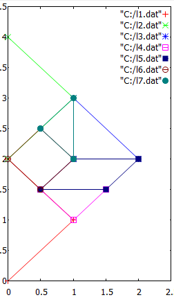
I used the symmetry of each puzzle piece and a heuristic for choosing which puzzle piece to fit in reducing the number of permutations used for solving a Tangram.
For the puzzle piece symmetry, I used that the square is completely symmetric so only its first line segment needs to be used when fitting it. The triangle pieces are only partially symmetric so two of their three line segments need to be tried.
The below figure illustrates the symmetry of the square:
I used two heuristics for which pieces to try fitting, first try larger pieces before smaller ones and two skip a piece if another identical piece has already failed to be fitted (there are two identical small triangles and similarly two identical large triangles).
With the above two optimizations it takes ~1min to solve a Tangram. Without the optimizations the algorithm did not complete for the Tangrams I tried.
River Flow Forecasting Using Support Vector Machines
Over the past few months I and a colleague (Brian Wallace) have been working on a river flow forecasting paper. A draft version is available @ River Flow Paper.
The goal of our work was to beat the current forecast methods used by the Department of Water Resources for the April through July American River flow. The Department of Water Resources uses an aggregation of human judgement and linear regression equations for generating their forecasts. Given their methods they are surprisingly hard to beat!
We spent a few months trying different Machine Learning methods with little success. Many of the methods we tried resulted in forecasts that were significantly worse than the current forecasts, a few methods such as a properly trained neural network gave forecasts that were comparable to the current forecasts. Finally, I decided to use a Support Vector Machine (SVM) for producing forecasts, after testing a large combination of parameters the forecasts started being significantly better than the current ones.
The data we used for generating forecasts is available online @ https://github.com/bjwbell/California-Water-Runoff-Forecasting. The takeaway message is that we improved the forecast relative error from ~65% to ~48%. The below table shows the forecasts for the last 10 years.
| Year | Actual (AcreFt) | Predicted (AcreFt) | |Error| (AcreFt) |
| 2001 | 552,626 | 689,472 | 136,846 |
| 2002 | 973,817 | 1,028,681 | 54,864 |
| 2003 | 1,354,434 | 459,476 | 894,957 |
| 2004 | 632,159 | 713,440 | 81,281 |
| 2005 | 2,003,878 | 1,844,360 | 159,517 |
| 2006 | 2,622,387 | 2,315,193 | 307,193 |
| 2007 | 522,651 | 293,256 | 229,394 |
| 2008 | 674,287 | 800,080 | 125,793 |
| 2009 | 1,068,327 | 1,253,523 | 185,196 |
| 2010 | 1,486,780 | 1,023,649 | 463,130 |
| Mean | 1,189,135 | 1,042,113 | 263,817 |
| Root mean squared error | 355,856 | ||
| Relative absolute error | 48.65% | ||
| Root relative squared error | 54.14% | ||
The forecasts currently used by the Department of Water Resources produced relative errors of 63.82% and root relative squared errors of 69.15%. Using modern methods for SVM’s gave us an increase in relative accuracy of over 15%! This was a fantastic result and shows the large payoff in keeping up with the state of art for something as ordinary as river flow forecasting.
